Hessian-Schatten Total Variation
@BIG.EPFL

Suppose you have a dataset \({\mathrm D}\) that consists of sequence of \(M\) images of mountains together with their prominence in meters (I'll just call it height, because being precise about mountain geography is not the point here). Mathematically, we write this statement as \({\mathrm D} = \lbrace{\mathbf x}_m, y_m\rbrace _{m=1}^M\), where each datapoint \(({\mathbf x}_m, y_m)\) is an image-height pair, as depicted below.

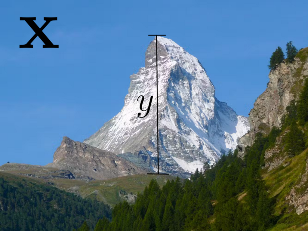
In supervised learning, our goal is to find a model \(f\) that predicts fairly well the height \(y_m\) of each mountain in our dataset from its depiction \({\mathbf x}_m\) (mathematically, \(f({\bf x}_m) = \hat{y}_m \approx y_m\)) 1, and that is able to generalize to new inputs: that is, that can accurately predict the heights of mountains from their respective images even when it has notfitting seen those images before in the training data.

In general, this is a very difficult task to solve because even though there are infinite models that fit the data well enough, very few of them actually make sense and are able to generalize. To tackle this issue, we need to introduce some constraints.

First, if we know something about the data distribution, then we can use that information. For example, if the data is the result of a linear mapping plus some measurement noise (mathematically, \(y = {\mathbf w}^T{\mathbf x} + b + \epsilon\)), then we can just search within this family of linear models; in this way, an a priori complicated problem is reduced to a simple one of finding just a few parameters (\({\mathbf w}\) and \(b\)). Alternatively, we might restrict ourselves to a family of models that we know to contain elements that perform well for similar tasks and introduce some information about what kind of models we're looking for in the form of regularization. This serves to make the problem solvable or to favor models that can generalize well 2. A very common practice is to use regularization terms favor simple models from the search space. This follows from the Occam's razor principle: as long as it can do the job, the simpler, the better. Simple models have the advantage of being lighter (ocupying less memory), faster, and being more robust—in that small or irrelevant changes in the image are less likely to screw up the predictions 3. Moreover, they are more are more explainable/interpretable: if they make a prediction error, we have a better chance of actually understanding what went wrong (*cough* ChatGPT *cough*) 4.

A family of models that has had a lot of success in the past few years are neural networks, which are part of the larger family of continuous and piecewise-linear functions (functions whose graph is composed of straight-line segments like this 📉) 5. But left to their own devices, neural nets lead to a very large number of linear regions, which makes them less robust and interpretable.

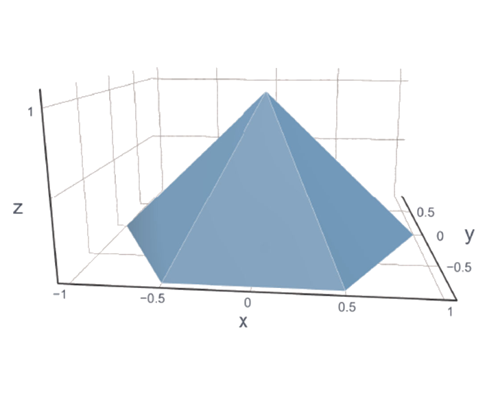
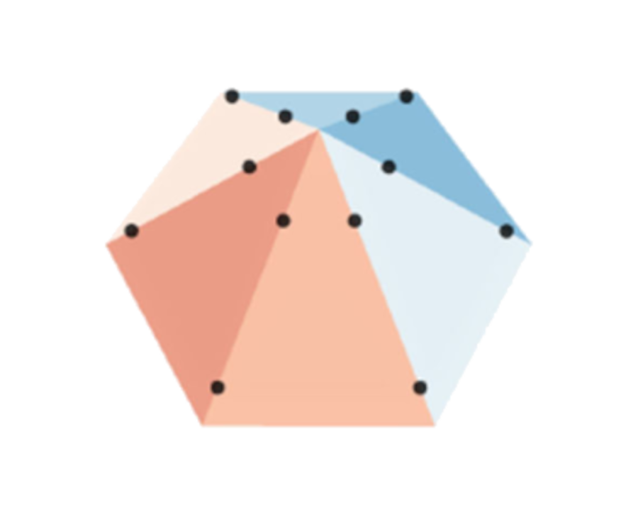
In this project, my colleagues at the Biomedical Imaging Group and I developed a method for learning continuous and piecewise-linear models characterized by few regions and a clear relationship with their parameters, rendering them interpretable. To achieve this, we employed a novel regularizer known as Hessian-Schatten Total Variation, designed to enforce sparse second derivatives, and restricted our search to a family of models composed of 'lego pieces' (basis functions) called box splines. In the following image you can see (on the left) one of these lego pieces, and (on the right) an example of a learned model that (in simple terms) results from placing different lego pieces with different heights at different locations.

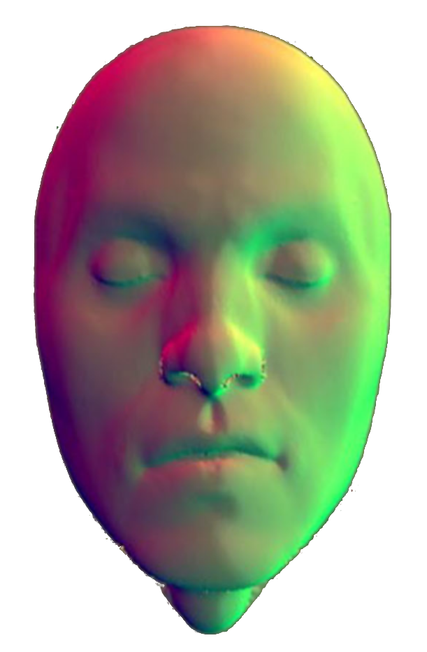
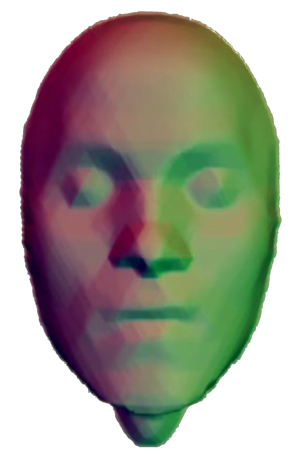
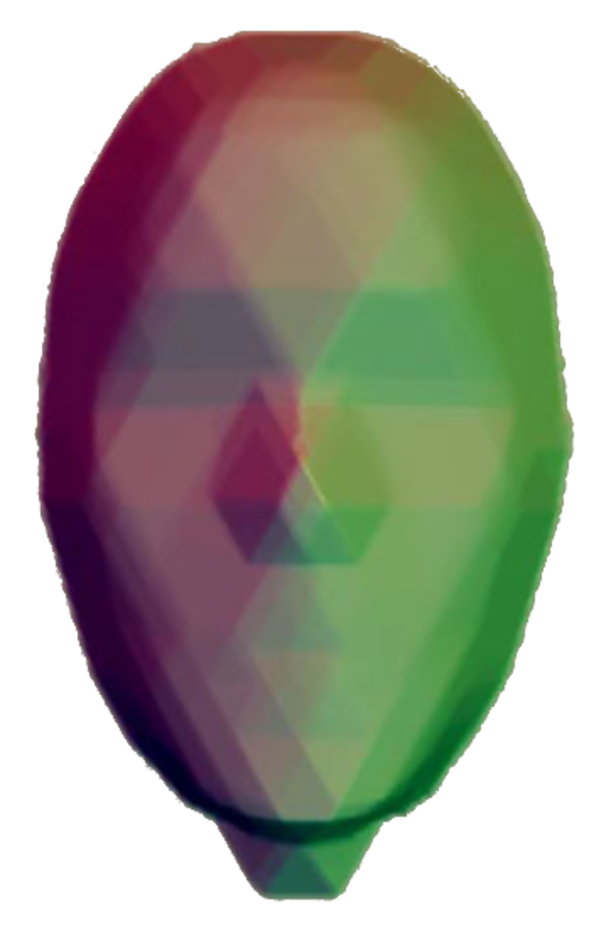
With this method we are able to regulate the level of simplicity (sparsity) in our models by adjusting a single parameter—the regularization weight. This is shown in top image in this page, where we trained our models on a face dataset with \(M = 5000\) samples. On the left, you can see the ground-truth; in the middle and right, you can see our learned models with different regularization weights, respectively. The model in the middle, which has a lower regularization weight, can fit the data better but has more linear regions than the model on the right.

Publications

Impact

This work relates to three papers that, in total, have been cited over 19 times in the scientific literature. In particular, these results were used in two papers [1, 2] of mathematician Luigi Ambrosio, a leading expert in the calculus of variations and geometric measure theory, and doctoral advisor of Fields Medal winner Alessio Figalli.

Code & Tech Stack

The code for this project can be found in this Github Repository. Here, I outline a few technologies that were used:

• Python: Programming language.
• Pytorch: Deep learning framework.
• Bash: Unix shell and command language.

Acknowledgments

I would like to thank my supervisor, Shayan Aziznejad, and Professor Michael Unser for their kindness and insight.